Sigmoid Function

What exactly is a sigmoid function? How does it convert the continuous linear regression line to S curve ranging from 0-1?

Let us try and understand this...

The mathematical equation for the sigmoid function is:-

P=1/(1+$exp^-$ $^Z$)

where Z is the linear regression line given by $b_0 + b_1x_1 + b_2x_2 + … b_nx_n$ or log(odds).

Let’s derive the equation for the sigmoid curve.

Consider a linear regression line given by the equation:

Y= $b_0 + b_1x_1 + b_2x_2 + b_3x_3 + ………….$ -Equation(1)

Let’s say instead of y we are taking probabilities (P) which will be used for classification.

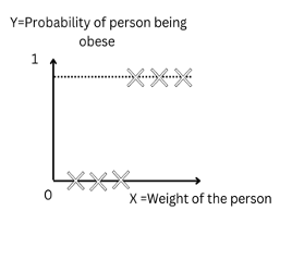Figure-(1)

The RHS(Right-hand side) of the equation(1) can take values beyond (0,1). But we know that the y(probability) will always be a value in the range (0,1).

To take control of this first we use odds instead of probability.

Odds:- The ratio of the probability of success to the probability of failure. Odds = P/1-P

So, the equation (1) can be written as:- P/1-P= $b_0 + b_1x_1 + b_2x_2 + b_3x_3 + ………….$

Now, the odds or P/1-P will take values between (0,$\infty$) as 0 <= P <= 1 but we don’t want a restricted range.

Modelling a variable with a limited range can be difficult.

Logistic regression requires a large amount of data points for a good classification model. To overcome this we use the log of odds transformation, which has an extended range and transforms the Y-axis from negative to positive infinity."

Since odds go from (0, $\infty$) log(odds) will go from (-$\infty$,+$\infty$).

Finally, the equation(1) after taking the log(odds) becomes

log(P/1-P)= $b_0 + b_1x_1 + b_2x_2 + b_3x_3 + ………….$ Equation(2)

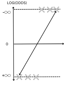Figure-(2)

Taking the exponent on both sides in equation(2) and solving for P(which is the probability given by the sigmoid curve) we will get:

P = 1/(1+$exp^-$ $^Z$), Z = $b_0 + b_1x_1 + b_2x_2 + b_3x_3 + …. b_nx_n$ or log(odds) - Equation(3)

Which is our sigmoid function.

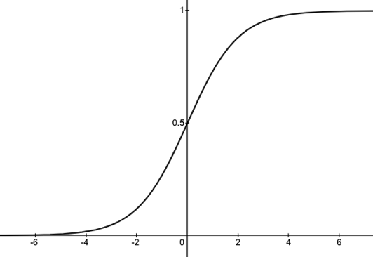Figure-(3)

If ‘Z’ or log(odds) goes to infinity, Y(predicted)/P will tend to 1 and if ‘Z’ goes to negative infinity, Y(predicted)/P will tend to 0.

Data is first projected into a linear regression line $b_0 + b_1x_1 + b_2x_2 + b_3x_3 + … b_nx_n$ or log(odds) from equation(2) to get the log(odds) values for each data points which is then fed as an input to the logistic/sigmoid function 1/(1+$exp^-$ $^Z$) for predicting the outcome. That’s the reason we use regression in ‘logistic models’ even when it’s used for solving classification problems.

In this way, the sigmoid function transforms the linear regression line(log(odds)) into an S-shaped curve which gives the probability of the categorical output variable ranging between (0,1). Based on a certain cut-off probability (default 0.5), any data lying above the cut-off probability will be considered 1 and data lying below the cut-off probability will be considered 0.

Cost Function

The cost function in linear regression is MSE (Minimum Squared Errors) given by the equation

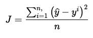Figure-(4)

where ŷ is the Linear Regression line (Predicted) and $y^i$ is the actual value.

On plotting the cost function MSE we get a convex graph having a global minimum. Hence, we can optimize the cost function or reduce the error (Minimum MSE) in the linear regression model via the gradient descent algorithm.

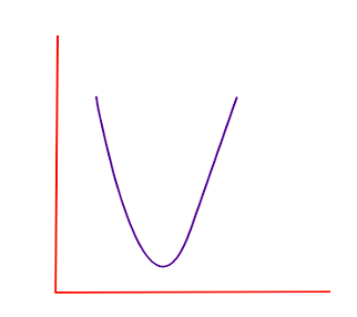Figure-(5)

In the case of logistic regression y(Predicted) or ŷ is given in terms of probability P=1/(1+e$xp^-$ $^Z$), where z = $b_0 + b_1x_1 ……b_nx_n$ or log(odds) If we apply this to the cost function J of the linear regression, we will obtain a non-convex graph with multiple local minima, making it difficult to optimise the cost function.

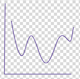Figure-(6)

To overcome this problem, we use another cost function called log loss or binary-cross-entropy loss for logistic regression defined as:

$Cost(h_\theta(x),y) = - ylog(h_\theta(x)) - (1 - y)log(1 - h_\theta(x)) ---Equation (4)$

In the above equation, $h_\theta(x)$/ŷ/P is the predicted value/probability and y is the actual value 0/1.

In Equation (4),

Cost($h_\theta(x)$, y) =

= - log($h_\theta(x))$, if y=1

= - log (1- $h_\theta(x))$, if y=0

For y=1

Log loss/Cost Function 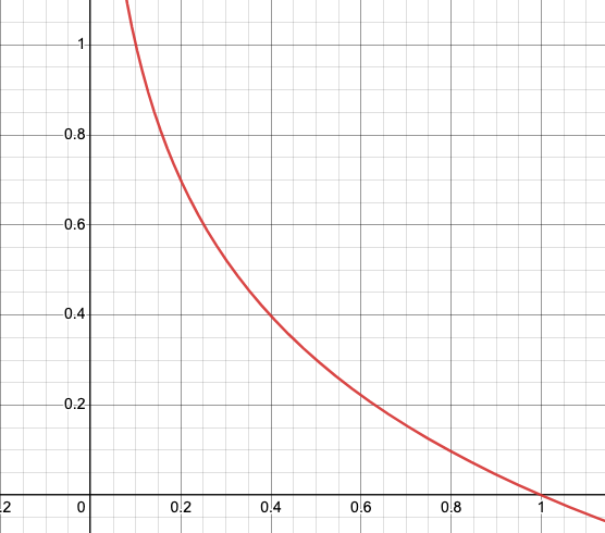$h_\theta(x)$ Figure-(7)

It is clear that when y (actual value) =1 and $h_\theta(x)$ (predicted value) = 1 then the cost function=0 and when y=1 and $h_\theta$(x)=0 then the cost function is infinite since it’s a case of incorrect classification.

Similarly, when y=0

Log loss/Cost Function 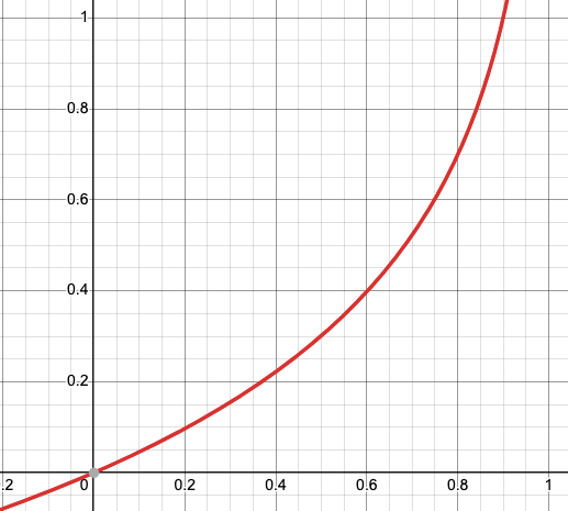$h_\theta(x)$ Figure-(8)

It is clear that when y (actual value) =0 and $h_\theta(x)$ (predicted value) = 0 then the cost function = 0 and when y = 0 and $h_\theta(x)$=1 then the cost function is infinite since it’s a case of incorrect classification.

On combining both graphs we will get a convex graph with one local minimum (Point of intersection) helping us to optimize the cost function or reduce the error in logistic regression model via the gradient descent algorithm.

Log loss $h_\theta(x)$ Figure-(9)

Maximum Likelihood Estimation(MLE)

Maximum likelihood estimation (MLE) is a statistical method used to estimate the parameters of a model such that it maximizes the likelihood of the observed data or in other words, the parameters that best fit or best explain the observed/actual data. Best fit is achieved when we get a distribution/curve that is as close as possible to the actual data points.

Let’s understand the concept with the example of obesity:

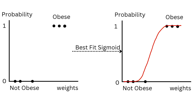Figure-(10)

Total 6 data points are given out of which $1^s$ $^t$ three points have P=0 or Not obese and the next 3 points have P = 1 and are obese(Y-axis) given the weights of the different persons(X-axis). The best fit sigmoid curve is drawn for the above data points.

We achieve this best-fit sigmoid curve in 3 steps:

• 1st step: log(odds) transformation

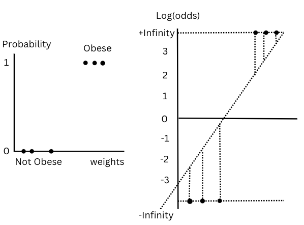Figure-(11)

The transformation from probability to log(odds) changes the Y axis from (0-1) to (-$\infty$ --- +$\infty$). Now we project the data points into the log(odds) linear line which gives the log(odds) value for each sample.

2nd step: log(odds) is passed as an input to the sigmoid function.

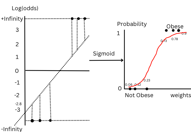Figure-(12), Line ‘A’

Log(odds) for each sample is passed as an input to the sigmoid function to give the respective probabilities of being obese. The probability given by the sigmoid function is 1/(1+exp(-Z)) where Z=log(odds).

For the first 3 data points log(odds) values are -2.8, -2 and -1.2 and probability given by sigmoid function will be 0.06,0.12 and 0.23.

Similarly for the next 3 data points log odds are 1,1.3,2.2 the probability will be 0.73,0.78 and 0.9

Likelihood of the data given this sigmoid curve will be:

$(1-0.06)*(1-0.12)*(1-0.23)*(0.73)*(0.78)*(0.9)=0.33$

Log-Likelihood will be log(0.35)= -0.48.

3rd step: Keep on rotating the log(odds) until we achieve maximum likelihood.

Now, let’s rotate the orientation of the log(odds)

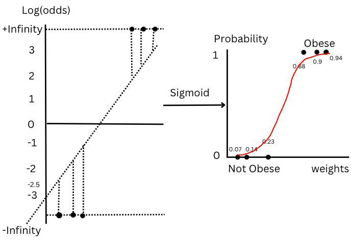Figure-(13), Line ‘B’

First 3 data points have log(odds) values as -2.5, -1.8 and -1.2, the probability will be 0.07,0.14 and 0.23.

For the next 3 data points log(odds) values are 2, 2.2 and 2.8, the probability will be 0.88,0.9 and 0.94.

Likelihood of the data given this sigmoid curve will be:

$(1-0.07)*(1-0.14) *(1-0.23) *(0.88) *(0.9) *(0.94)=0.45$

Log-Likelihood will be log(0.45)= -0.34.

The log-likelihood of line B(-0.34)>A(-0.48) which is justified as line B's sigmoid curve is much closer to the actual outcomes than line A’s sigmoid.

We keep on rotating the log(odds) line till we get the maximum log-likelihood or the sigmoid curve that is as close as possible to all the data points.

Summary

We are interested in finding the best fit S curve for given data points in logistic regression. The sigmoid function in logistic regression gives the Probability(P)=1/(1+exp(-Z) where Z= log(odds).

The goal of using maximum likelihood estimation in logistic regression is to find the model's parameters or log(odds) such that it maximizes the likelihood of observing the actual outcomes in the dataset. It does this by adjusting the log(odds) iteratively until the predicted probabilities given by sigmoid curve align as closely as possible with the actual outcomes. Adjusting the log(odds) changes the log-likelihood of the data for a sigmoid curve. We choose the sigmoid curve with maximum log-likelihood which helps in getting the best fit sigmoid curve for the data.

In simple terms, maximum likelihood in logistic regression finds the best values for the model's parameters(log(odds)) that make the predicted probabilities(sigmoid curve) as close as possible to the actual outcomes in the dataset.