LINEAR REGRESSION

In the previous blog, we have looked at different types of regression. Let’s begin by understanding the simple and most popular machine learning algorithm which is Linear Regression.

Introduction

Linear Regression is used for modelling a linear relationship between the dependent variable(Y) and one or more independent variables(X). Linear regression is a powerful tool which helps in making predictions for continuous variables like housing prices, sales of a product, weather forecasting etc.

Types Of Linear Regression

Based on the number of independent variables(X) we can categorize linear regression into mainly two types: -

• Simple Linear Regression: In simple linear regression we have only one independent variable(X) and one dependent variable(Y). In simple linear regression, a straight line which best fits the data is used for representing the relationship between the variables.
• Multiple Linear Regression: In multiple linear regression we have more than one independent variable(X) and one dependent variable(Y). In multiple linear regression, we find a hyperplane which best fits the data.

Let us try and understand the very basic type of regression which is ‘Simple linear regression’.

Simple Linear Regression

The equation for simple linear regression in which there is one independent variable(X) and one dependent variable(Y) will be a straight line which best fits the data.

We will be using the equation of a line in the slope-intercept form which is: -

$Y = a1*x + a0$

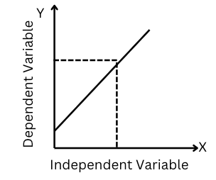
Figure-(1)

Where :- Y is the dependent variable, a1 is the linear regression coefficient or slope of the best-fit line and a0 is the intercept of the line.

There can be two major possibilities for a linear regression line: -

1. Positive Linear Regression Line:

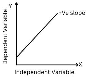
Figure-(2)

If the slope ‘a1’ (linear regression coefficient or slope of the best-fit line) in the equation, is positive (a1>0) then the dependent variable y will have a positive or direct relationship with the independent variable(x). Hence, the dependent variable(Y) will increase with the increase in the independent variable(x).

2. Negative Linear Regression Line:

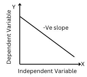
Figure-(3)

If the slope ‘a1’ (linear regression coefficient or slope of the best-fit line) in the equation, is negative (a1<0) then the dependent variable y will have a negative or inverse relationship with the independent variable(x). Hence, the dependent variable(Y) will decrease with the increase in the independent variable(x).

Let us have a look at the simple linear regression line and understand some of the important concepts associated with it.

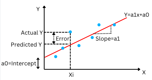
Figure-(4)

In the above graph, we can see that there are data points (scattered) blue in colour. The red line here is the linear regression line whose equation is given by

$Y = a1*x + a0$

The goal here is to get the linear regression line which best fits the given data. The line will be able to best fit the data if the residuals/error terms (e) above are minimum (least error) or we can say that the scatter data points will be close enough to the regression line.

The residuals/error term is the difference between the actual and predicted values (linear regression lines).

Error term= $Y_{actual} - Y_{predicted}$

Once we are able to get the linear regression line, we are ready with making predictions for the unseen data. From the equation in the linear regression line, we substitute for the unseen data(x) and get the corresponding target variable(Y).

But how do we get these best-fit regression line coefficients which are a1 and a0??

Imagine a line in 2D plane(X-Y) with coefficients a1 and a0. As we change the value of the coefficients a1 and a0 we can see that a different linear regression line with different slopes and intercept is generated. By changing the value of these coefficients, we will be able to arrive at such an orientation of the linear regression line which has the least error or minimum residuals.

Cost Function

With the help of the cost function, we are able to determine the coefficients a1 and a0 which helps in obtaining a line that best fits the given data points.

In linear regression, we use MSE (mean squared error) as the cost function. MSE is the mean/average of the squared errors that resulted between the actual values and predicted values.

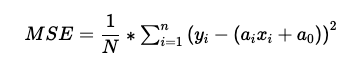
N = Total no of observations/data points (blue points). Yi = Actual value. YPredicted = Predicted value=.

By utilizing this cost function MSE we will be able to update coefficients a1 and a0 such that MSE attain its minima. If we have the minimum MSE, the error/residuals will also be small. This way, we get a linear regression line that best fits the given data points.

Performance/Evaluation Metrics

The evaluation metrics in linear regression are measures used to assess the performance of the model. It is used for determining how well a particular linear regression model or algorithm is working. The methods used for finding the best model out of all the possible models are called optimization methods/techniques.

Some of the most commonly used evaluation metrics in linear regression are:-

• Mean squared error (MSE): MSE is the mean/average of the squared errors that resulted between the actual values and predicted values. A model with a lower MSE value will be a good-performing model.

• Root Mean squared error (RMSE): Root mean squared error is the square root of MSE which is RMSE= √MSE. It should also be lower for a good-performing model.

• The goodness of Fit(R2): Goodness of fit of a model or R2 value is the ratio of the explained variation/Total variation. R2 is a value between 0-1. R2 close to the value of 1 indicates that the regression model is able to explain a large proportion of the variance in the dependent variable and hence the difference between the predicted value and the actual value is smaller.

The high R-squared value determines the lower difference between the predicted and actual values and hence represents a good model.

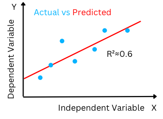
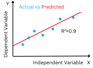
Figure-(5)

Assumptions in Linear Regression:

Some of the assumptions that linear regression makes for the best prediction from the given dataset are:

• Linearity: Linear Regression makes the assumption that the relationship between dependent and independent variables is linear in nature.
• Homoscedasticity: Homoscedasticity or homogeneity of variances, is an assumption that the variance of the residuals, error terms (the difference between the actual and the predicted value)- is equal or constant for all independent variables.
• Normality: The error terms are normally distributed in nature with the mean equal to the value of zero.
• Little or No Multicollinearity: Linear regression makes the assumption that there is no significant correlation (zero or less multicollinearity) between the independent variables. A multicollinearity (high correlation) present between the independent variables will fail us to understand the effect of individual independent variables on the target or dependent variable.
• No autocorrelations: There is no auto-correlation between the residuals and error terms (the differences between the predicted and actual values).

Biased or inefficient coefficients will be estimated for the best fit if the following assumptions are not correct. Therefore, it is important to check these assumptions before analysing the results of linear regression.