INTRODUCTION:

In this blog, we will explore the effectiveness of decision trees and random forests in predicting customer churn, conducting a performance evaluation.

Importing Essential Libraries:

import numpy as np
import pandas as pd
import matplotlib.pyplot as plt
import seaborn as sns

Reading the data:

df=pd.read_csv('customer_churn-2.csv')

EXPLORATORY DATA ANALYSIS(EDA):

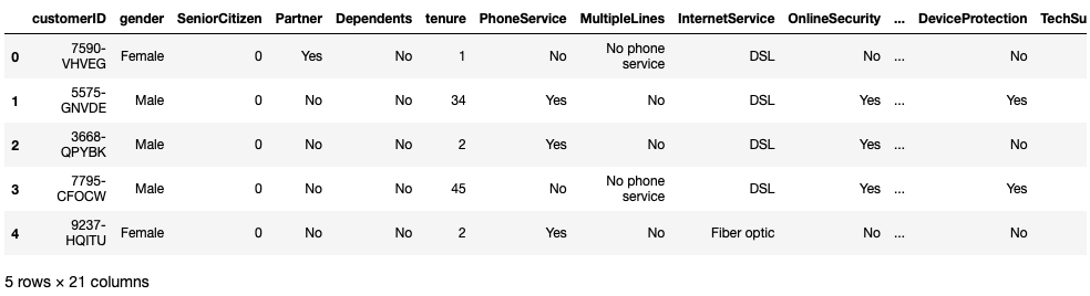
df.head()

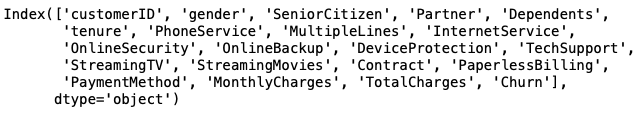
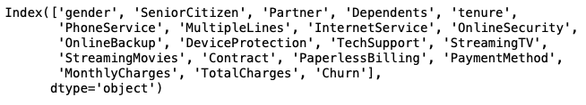
df.columns

df.info()

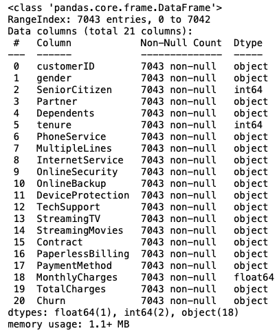The total charges must be of a numeric datatype, but due to the possible presence of some strings, it may become an object.

df['TotalCharges']=pd.to_numeric(df['TotalCharges'],errors='coerce') 

Coerce converts the string to nan.

df['TotalCharges'].dtype
dtype('float64')

Checking the null values in the dataset:

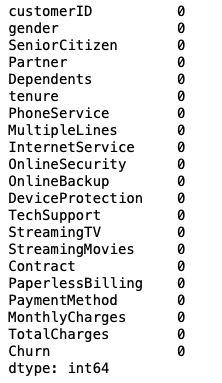
df.isna().sum() 

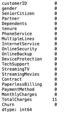
11 values of column 'TotalCharges' are converted into nan because of errors=coerce as it cannot be converted to numeric.

Now, we can drop 11 rows since this number is relatively small compared to the total of 7043 rows.

df.dropna(inplace=True)
df.isna().sum()

df.shape
(7032, 21)

Since customer ID is unique to each customer and does not contribute to predicting the 'Churn' outcome, we will drop this column.

df.drop(columns=['customerID'],inplace=True)
df.columns

Statistical inference for numerical columns:

df.describe()

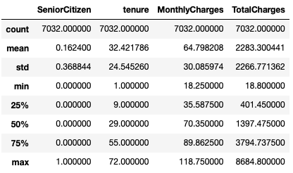
We need to convert non-numeric and categorical columns with labels/strings such as 'Yes' and 'No,' as well as other columns containing strings, into numeric types. Non-numeric columns are not suitable for classification algorithms like logistic regression or tree-based models, as these models rely on mathematical computations such as sigmoid, predict_proba, entropy, and gini-impurity for classification.

Using MAP/Label Encoding Function For Conversion:

df['gender']=df['gender'].map({'Female':1,'Male':0})
df['Partner'] = df['Partner'].map({'Yes': 1, 'No': 0})
df['PhoneService']=df['PhoneService'].map({'Yes':1,'No':0})
df['Dependents'] = df['Dependents'].map({'Yes': 1, 'No': 0})
df['MultipleLines']=df['MultipleLines'].map({'No phone service':0, 'No': 1, "Yes": 2})
df['InternetService']=df['InternetService'].map({'DSL':0, 'Fiber optic':1, 'No':2})
df['OnlineSecurity']=df['OnlineSecurity'].map({'Yes':1, 'No':0, 'No internet service':2})
df['OnlineBackup']=df['OnlineBackup'].map({'Yes':1, 'No':0, 'No internet service':2})
df['DeviceProtection']=df['DeviceProtection'].map({'Yes':1, 'No':0, 'No internet service':2})
df['TechSupport']=df['TechSupport'].map({'Yes':1, 'No':0, 'No internet service':2})
df['StreamingTV']=df['StreamingTV'].map({'Yes':1, 'No':0, 'No internet service':2})
df['StreamingMovies']=df['StreamingMovies'].map({'Yes':1, 'No':0, 'No internet service':2})
df['Contract']=df['Contract'].map({'Month-to-month':0, 'One year':1, 'Two year':2})
df['PaperlessBilling']=df['PaperlessBilling'].map({'Yes':1, 'No':0})
df['PaymentMethod']=df['PaymentMethod'].map({'Electronic check':1, 'Mailed check':0, 'Bank transfer (automatic)':2, 'Credit card (automatic)':3})
df.dtypes

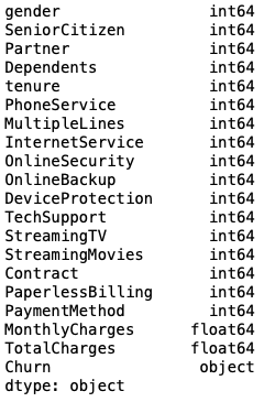
Now, after mapping the non-numeric columns, you can observe that the data types of all input features are numerical. Therefore, this data is well-suited for any classification problem.

DATA VISUALIZATION:

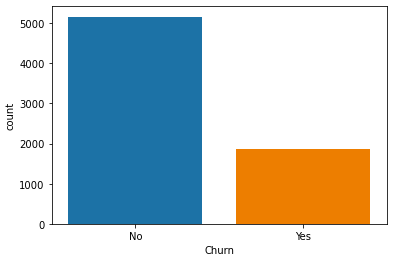
sns.countplot(x=df['Churn'],data=df)
plt.show()

df.Churn.value_counts(normalize=True)

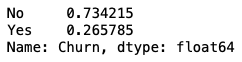The percentage of people leaving the telecom service is 26.5%, while the percentage of those not leaving is 73.5%. Hence, the dataset is imbalanced.

plt.subplots(1,2,figsize=(16,6))
plt.subplot(1,2,1)
sns.scatterplot(x='TotalCharges',y='tenure',hue='Churn',data=df)
plt.subplot(1,2,2)
sns.scatterplot(x='MonthlyCharges',y='tenure',hue='Churn',data=df)
plt.show()

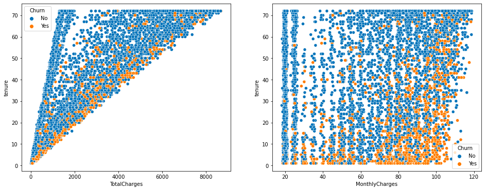
As total charges increase, the churn rate also shows a slight increase. In the second plot, where monthly charges are rising (80-100) and tenure is low, the churn rate is also increasing.

plt.figure(figsize=(15,12))
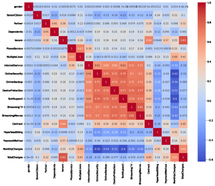
sns.heatmap(df.corr(),annot=True,cmap='coolwarm')  #annot=True gives the correlation for columns mathematically.
plt.show()

MODEL BUILDING:-

Splitting the dataset into input features (X) and output target (churn) values (Y)
X=df.iloc[:,:-1]

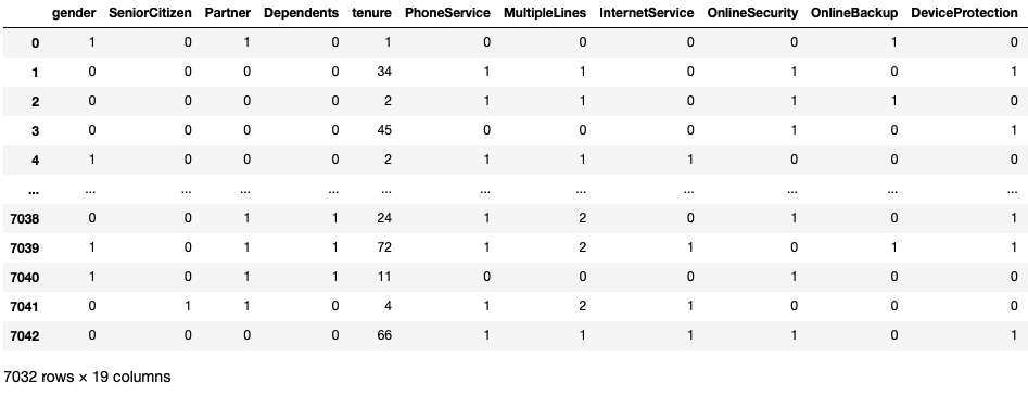
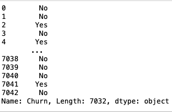
Y=df.iloc[:,-1]
Y

Importing train-test split for splitting the data into training and testing/unseen data for the model:

from sklearn.model_selection import train_test_split
x_train,x_test,y_train,y_test=train_test_split(X,Y,random_state=0,test_size=0.2) 

Setting test_size=0.2 implies that 20% of the data (approximately 1407 out of 7043) will be used for testing the model, while the remaining 80% of the data will be used for training the model.

print(x_train.shape)
print(x_test.shape)
print(y_train.shape)
print(y_test.shape)

(5625, 19)
(1407, 19)
(5625,)
(1407,)

Decision Tree algorithm:

from sklearn.tree import DecisionTreeClassifier  

#Creating an instance of Decision Tree:  
dt=DecisionTreeClassifier()  

#Training the decision tree model:
dt.fit(x_train,y_train)
DecisionTreeClassifier()  

#Making predictions on unseen/test data.
y_pred=dt.predict(x_test)  

Importing Evaluation Metrics for Classification:

from sklearn.metrics import accuracy_score,confusion_matrix
print(accuracy_score(y_test,y_pred))
print(confusion_matrix(y_test,y_pred))  

0.7391613361762616
[[847 191]
 [176 193]]

Random Forest Algorithm:

from sklearn.ensemble import RandomForestClassifier
rf=RandomForestClassifier()
rf.fit(x_train,y_train)
RandomForestClassifier()  

#Making predictions on unseen/test data:
y_pred_rf=rf.predict(x_test)


#Importing Evaluation Metrics for Classification:
from sklearn.metrics import accuracy_score,confusion_matrix
print(accuracy_score(y_test,y_pred_rf))     
print(confusion_matrix(y_test,y_pred_rf))  

0.7874911158493249
[[926 112]
 [187 182]]

Conclusion:

We can observe that the Random Forest model has effectively reduced variance and improved accuracy on the testing data. The accuracy for the Decision Tree model on the testing data is 73%, while the Random Forest model achieves an accuracy of 78%