INTRODUCTION

In this blog, we will look at the housing dataset and use linear regression to predict the price of a house based on different factors.

Importing Essential Libraries:

#Importing numpy for computations
#Importing matplotlib for visual representation

import numpy as np
import matplotlib.pyplot as plt

Ignoring Warnings:

import warnings
warnings.filterwarnings('ignore')

Importing the numpy,pandas and Visualisation package:

import numpy as np
import pandas as pd
import matplotlib.pyplot as plt 
import seaborn as sns

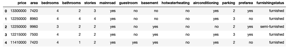
Reading of the housing data

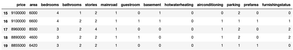
housing=pd.read_csv('Housing.csv')
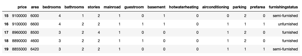
housing.head()

DATA INSPECTION:-

#No of rows and columns in the dataset
housing.shape
(545, 13)


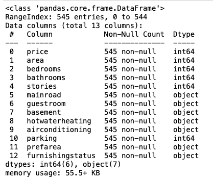
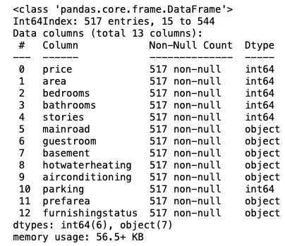
#Columns,non null counts and their data type
housing.info()

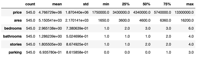
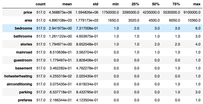
#Descriptive statistics of data

housing.describe().T

DATA CLEANING:-

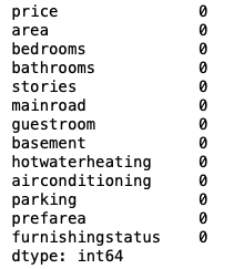
#Checking the total null values in each column of the dataset.
housing.isnull().sum()

Outliers Analysis:-

fig, axs = plt.subplots(2,3, figsize = (10,5))
sns.boxplot(housing['price'], ax = axs[0,0])
sns.boxplot(housing['area'], ax = axs[0,1])
sns.boxplot(housing['bedrooms'], ax = axs[0,2])
sns.boxplot(housing['bathrooms'], ax = axs[1,0])
sns.boxplot(housing['stories'], ax = axs[1,1])
sns.boxplot(housing['parking'], ax = axs[1,2])
plt.show()

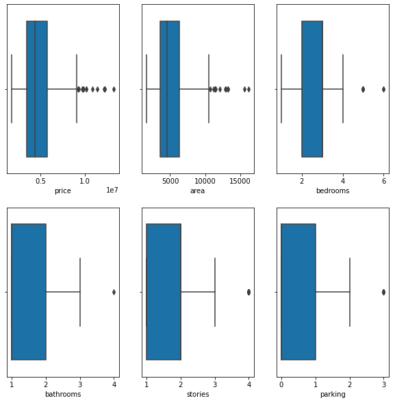
we can clearly see from the above box plot(which shows the distribution of data column wise) that the price and area has sufficient outliers.

#Outliers treatment for price:-
Q1=housing['price'].quantile(0.25)
Q3=housing['price'].quantile(0.75)
IQR=Q3-Q1
housing=housing[(housing['price']>=Q1-1.5*IQR) & (housing['price']<=Q3+1.5*IQR)]


#Outliers treatment for AREA:-

Q1=housing['area'].quantile(0.25)
Q3=housing['area'].quantile(0.75)
IQR=Q3-Q1
housing=housing[(housing['area']>=Q1-1.5*IQR) & (housing['area']<=Q3+1.5*IQR)]


#Clearly some of the rows in the housing dataset are removed containing outliers of price and area.
housing.shape
(517, 13)

housing.info()

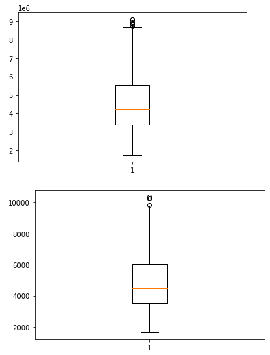
Analysis after treatment of outliers:

plt.boxplot(housing.price)
plt.show()
plt.boxplot(housing.area)
plt.show()

EXPLORATORY DATA ANALYSIS:-

Let us know understand the data:-

1.Checking for multicollinearity among the independent variables.

2.How each independent variables is related to the target variabe.

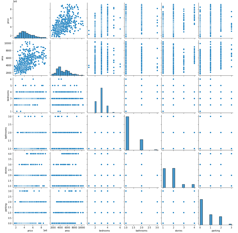
#Visualizing the numerical variables:-
sns.pairplot(housing)
plt.show()

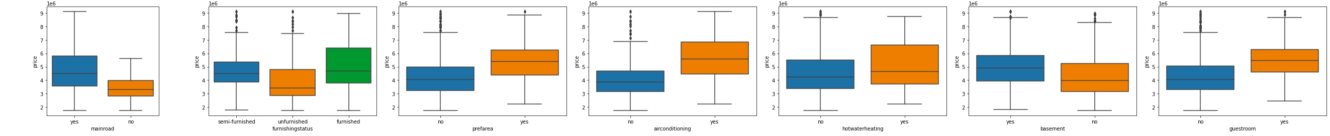
#Visualizing the categorical variables:-
for i in housing.columns:
  if(housing[i].dtype!=int):
    sns.boxplot(x=i,y='price',data=housing)
    plt.show()

DATA PREPARATION & PREPROCESSING:-

Many of the independent variables are categorical in nature.The linear regression has to find the best fit line via numerical methods. So we need to convert this categorical variables into numerical for doing the regression analysis:-

#From the above box plot we can clearly see that except the column furnishing status,rest all the categorical variables have yes or no values.
#so we give yes as 1 and no as 0.

for i in housing.columns:
  if( (housing[i].dtype!=int) & (i!='furnishingstatus') ):
    housing[i]=housing[i].replace({'yes': 1, "no": 0})
      
housing.head()

#All the categorical variables are converted into numerical values 0 and 1,except furnishingstatus.lets look us at unique value of furnishingstatus. 

housing.furnishingstatus.value_counts()

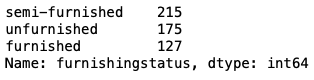
#We are converting semi-furnished,unfurnished and furnished to numerical variables using 0,1 and 2.
housing['furnishingstatus'].replace({'semi-furnished':0,'unfurnished':1,'furnished':2},inplace=True)

housing.head()

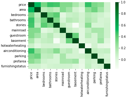
#we will be seeing correlation matrix using heatmap to see how the variables are related with each others.
sns.heatmap(housing.corr(),cmap='Greens')
plt.show()

from sklearn.preprocessing import MinMaxScaler
sc=MinMaxScaler()  #creating an object of MinMax Scaler
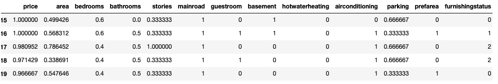
num_vars = ['area', 'bedrooms', 'bathrooms', 'stories', 'parking','price']
housing[num_vars]=sc.fit_transform(housing[num_vars])

housing.head()

housing.describe()

PREPARING THE INPUT X AND OUTPUT Y VARIABLES AND SPLITTING THE DATA INTO TRAIN AND TEST SET:-

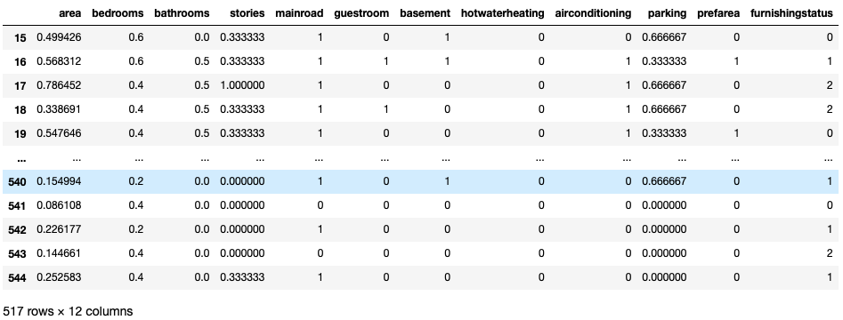
x=pd.DataFrame(housing.iloc[:,1:])
x

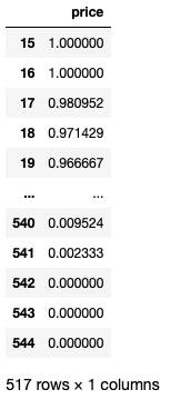
y=pd.DataFrame(housing.iloc[:,0])
y

from sklearn.model_selection import train_test_split
x_train,x_test,y_train,y_test=train_test_split(x,y,train_size=0.7,random_state=180)

x_train.shape
(361, 12)
x_test.shape
(156, 12)
y_train.shape
(361, 1)
y_test.shape
(156, 1)

Importing the linear regression and training(fit) the model:

from sklearn.linear_model import LinearRegression
linear_model=LinearRegression()
linear_model.fit(x_train,y_train)

Prediction of the output variable y by the model.

y_pred=linear_model.predict(x_test) 


#Y=m1x1+c1+m2x2+c2+m3x3+c3...and so on
#we will get the values of m1 and c1 by using linear_model.coef_ and by linear_model.intercept_. of the linear regression

Finding the linear model coefficients:

coef=linear_model.coef_  
col=housing.columns[1:]
coefficients=pd.DataFrame(coef,columns=col)
coefficients.T

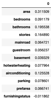
#we can clearly see that the area has the highest impact on the price of the house and neglecting mainroad,guestroom,basement,hotwaterheating and furnishing status as they have insignificant effects on price.

so, price=0.31area+0.2bathrooms+0.16stories+0.12airconditioning

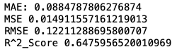
EVALUATION METRICS FOR MODEL PERFOMANCE:-

from sklearn import metrics
print('MAE:', metrics.mean_absolute_error(y_test,y_pred))
print('MSE',metrics.mean_squared_error(y_test,y_pred))
print('RMSE',np.sqrt(metrics.mean_squared_error(y_test,y_pred)))
print('R^2_Score',metrics.r2_score(y_test,y_pred))